
Author: David Max MA DPhil (2015-08-04)
Convergence requirements for Garrett's elliptic integral solver
This example explores numerical accuracy in solvers used in superconducting magnet design calculations.
In his publications M.W.Garrett describes an elliptic integral solver for calculating inductances, fields and forces in axisymmetric magnet systems [1].
The method relies on Gauss-Legendre quadrature, a type of numerical integration [2]. Here is a review of convergence requirements. Convergence is shown to depend on the order of the integration.
- Requirement for numerical integration over coil depth
- Numerical integration in outline
- Weights and abscissas for Gauss-Legendre quadrature
- Convergence requirements for the solver
- Example system: a 3T MRI magnet system
- Test-point locations
- Required Gauss orders
- Is elliptic integral computation the main source of errors?
On devices with wider screens a version of this webpage is available as a pdf document.
Requirement for numerical integration over coil depth
The magnetic field generated by either an idealised current loop (with infinitesimally small thickness in both the axial and radial directions) or of a current sheet (infinitesimal in the radial direction, but with finite length in the axial direction) can be computed fairly easily using analytical formulae.
For example, to find the magnetic flux density B generated by a circular current loop, the Biot-Savart rule can be employed.
Solving the above problem for a current sheet involves an integral in the axial direction that can be done analytically. However, when the coil has finite length and finite thickness in the radial direction, Garrett says that the required integral has no known analytical solution and must be evaluated numerically.
Numerical integration in outline
The numerical estimate of a definite integral is obtained by forming the weighted sum of integrand values at specific points along the integration scale. The resulting weighted sum must then be multiplied by the range of the integration scale. The key requirements are
- 1) an expression for the integrand y in terms of the dependent variables;
- 2) the integration range {a, b};
- 3) the locations along the integration scale, the abscissas, xi, where the integrand needs to be evaluated; and
- 4) the weights wi, i.e. the factors by which the integrand values need to be multiplied before forming the overall sum.
[If these requirements are met, a numerical integral can be formed quite easily using Excel's SUMPRODUCT worksheet function. Suppose range A1:A10 contains the abscissa values; range B1:B10 contains formulae to compute the integrand values for these abscissas; and range C1:C10 contains the weights. Then SUMPRODUCT(B1:B10, C1:C10) supplies the required weighted sum, which, multiplied by the integration range (b-a) gives the estimated value of the integral.]
The number of points used in computing the integral is the integration order n. In the Excel example, the integration order would be n = 10.
Weights and abscissas for Gauss-Legendre quadrature
Gauss-Legrendre quadrature is a standard method for performing numerical integration. This is a highly accurate method for evaluating integrals of this kind (for others, see e.g. [2], [3]).
An earlier version of the F77 routines used here took abscissas and weights directly from the tables in Abramowitz and Stegun [3]. Recently the code was modified to include abscissas and weights for n from 2 to 64 taken from Mike 'Pomax' Kamermans' webpage [4]. Many thanks to him for this material.
Although the Kamermans table goes up to n = 64, this study effectively extends the range of available values for n to 512 by splitting the study coil into five or eight equal depth shells.
Convergence requirements for the solver
Convergence requirements are a key consideration in numerical integration. Garrett warns of convergence problems for the solver when applied to locations near the ends of thick coils. Below is a summary of results on the effect of varying the integration order n on the apparent accuracy of the computed fields, based on a typical MRI magnet.
Example system: a 3T MRI magnet system
The calculations are based on coil 4 alone of the 3 tesla MRI magnet system from Liebel. For simplicity, coil 4 is set to operate at unit current (1 amp) and the other coils are left out of the calculations. The plots were all produced using R.
Test-point locations
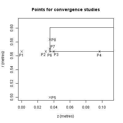 Five regions are considered here:
- Field at the origin
- Points on the inner coil radius, far from coil end
- Points on the inner coil radius, near the end of the coil
- Point P5
- Points on the end of the coil
Field at the origin
.png) On the plot the bands either side of 1.0 are equivalent to a discrepancy of 1 part per thousand.
On the plot the bands either side of 1.0 are equivalent to a discrepancy of 1 part per thousand.
The points are grouped by 'ndivs', the number of equal-depth shells into which coil 4 was divided for the calculations.
For the point at the origin, the axial field component Bz agrees closely with the value of the zeroth-order term in the zonal harmonic series. The zonals series gives A(0,0) = 0.002006944 T/A. At unit current, the elliptic integral solver also gives 0.002006944 T for the axial component Bz, so agreement is up to the 7th digit of the floating point result. Convergence is very rapid and n = 2 (i.e., two idealised sheet solenoids) is sufficient to give essentially the same result as n = 64. With n = 2, the discrepancy is already just a few parts in 108.
Points on the inner coil radius, far from coil end
.png) Away from the end-plane of the coil , the computed field also converges quickly. For point P4 the apparent error (discrepancy from the value obtained using 512 current sheets) is down to the order of a part in 107 with n = 4.
Away from the end-plane of the coil , the computed field also converges quickly. For point P4 the apparent error (discrepancy from the value obtained using 512 current sheets) is down to the order of a part in 107 with n = 4.
Points on the inner coil radius, near the end of the coil
.png) Nearer to the coil end-plane, the computed field converges more slowly. However, even for point P2, 5.1 mm from the end surface of the coil, with a single shell (ndivs = 1) the apparent error is down to the order of a part in 107 with n = 11.
Nearer to the coil end-plane, the computed field converges more slowly. However, even for point P2, 5.1 mm from the end surface of the coil, with a single shell (ndivs = 1) the apparent error is down to the order of a part in 107 with n = 11.
Point P5
.png) Well away from the coil inner radius, even in the plane of the coil end, computed fields converge quickly. Apparent error is of the order of a part in 107 with n = 3.
Well away from the coil inner radius, even in the plane of the coil end, computed fields converge quickly. Apparent error is of the order of a part in 107 with n = 3.
Points on the end of the coil
.png) Here convergence with increasing Gaussian order is slow.
Here convergence with increasing Gaussian order is slow.
Point P6, on the coil corner, is informative because being right on the inner edge of the coil, no integration abscissa ever coincides with it. The computed field modulus converges smoothly, approximately exponentially with increasing n.
.png) Point P7 was purposely chosen to be potentially pathological. P7 falls on the end of the coil but the radius is arbitrary. For points in end-zones Garrett recommends splitting the coil into at least two contiguous shells, with the field point located at the radius where the shells touch.
Point P7 was purposely chosen to be potentially pathological. P7 falls on the end of the coil but the radius is arbitrary. For points in end-zones Garrett recommends splitting the coil into at least two contiguous shells, with the field point located at the radius where the shells touch.
Convergence results for P7 show what may happen if these precautions are ignored. Although the computed field does gradually, erratically, converge to a steady value, an excessive number of sheet ('ideal') solenoids is required to bring the uncertainties down to reasonable levels.
.png) For point P8, midway down the end-face of coil 4, the computed field is apparently accurate at the level of 1 or 2 percent. This is clearly not a high level of accuracy but may still be tolerable for practical purposes. Peak fields will usually occur towards the middle of the inner surface of a coil. There, as convergence for P4 above shows, the computed field values are expected to be highly accurate with quite modest values for n.
For point P8, midway down the end-face of coil 4, the computed field is apparently accurate at the level of 1 or 2 percent. This is clearly not a high level of accuracy but may still be tolerable for practical purposes. Peak fields will usually occur towards the middle of the inner surface of a coil. There, as convergence for P4 above shows, the computed field values are expected to be highly accurate with quite modest values for n.
Convergence is quicker with 8 radial subdivisions (i.e., an even number of shells) than with 1 or 5 shells. The explanation for this effect seems to be that, for the odd numbers of shells, one of the abscissas may (almost) collide with the location of P8. This occurs despite a trap on very small values of Garrett's k in the Fortran that should force the routine to exit.
Required Gauss orders
Based on the calculations described here, the table below indicates the minimum number of current sheets to achieve pre-specified levels of convergence. These should be indicative of appropriate Gauss orders.
| point | 1 in 103 | 1 in 104 | 1 in 105 | 1 in 106 |
|---|---|---|---|---|
| P0 | 1 | 1 | 1 | 1 |
| P1 | 1 | 2 | 2 | 3 |
| P2 | 3 | 5 | 6 | 9 |
| P3 | 3 | 5 | 7 | 8 |
| P4 | 1 | 1 | 2 | 2 |
| P5 | 1 | 1 | 1 | 2 |
| P6 | 12 | 21 | 50 | 80 |
| P7 | 36 | 36 | 36 | 81 |
| P8 | 46 | 57 | 63 | 67 |
| P9 | 1 | 1 | 2 | 2 |
The results in the table are in general agreement with Garrett's recommendations. Only quite low Gauss orders are required in order to achieve high accuracy for many regions. Within end-zones the coil must be split radially into at least two shells (as in P8). Garrett used n up to 16 but says that up to four radial subdivisions were used in his programs. This seems to be equivalent to a possible limit of 64 current sheets, which accords well with the numbers shown for point P8. With tables going up to n = 64, a realistic target would be to achieve one part in 104 for the most difficult locations.
Is elliptic integral computation the main source of errors?
The answer to this question would seem to be clearly not.
Below is a table of the values for integrals K and E computed by G65ELL, the Fortran routine used by acrocephalus.com to compute Garrett's equations 18 to 21. Whereas Garrett says that the integrals can be computed to a few parts in 108, with double (i.e. eight-byte) precision, the errors are much smaller than this:
| alpha (rad.) | alpha (deg.) | K calc | K (table) | K error | E calc | E (table) | E error |
|---|---|---|---|---|---|---|---|
| 1.3963 | 80 | 3.1534 | 3.1534 | -3.80E-15 | 1.0401 | 1.0401 | 2.13E-16 |
| 1.4137 | 81 | 3.2553 | 3.2553 | -3.55E-15 | 1.0338 | 1.0338 | -8.59E-16 |
| 1.4312 | 82 | 3.3699 | 3.3699 | -3.16E-15 | 1.0278 | 1.0278 | -8.64E-16 |
| 1.4486 | 83 | 3.5004 | 3.5004 | -3.55E-15 | 1.0223 | 1.0223 | -4.34E-16 |
| 1.4661 | 84 | 3.6519 | 3.6519 | -5.35E-15 | 1.0172 | 1.0172 | 0.00E+00 |
| 1.4835 | 85 | 3.8317 | 3.8317 | -4.17E-15 | 1.0127 | 1.0127 | -4.39E-16 |
| 1.5010 | 86 | 4.0528 | 4.0528 | -8.99E-15 | 1.0086 | 1.0086 | -2.20E-16 |
| 1.5184 | 87 | 4.3387 | 4.3387 | -5.94E-15 | 1.0053 | 1.0053 | -8.84E-16 |
| 1.5359 | 88 | 4.7427 | 4.7427 | -1.27E-14 | 1.0026 | 1.0026 | -1.11E-15 |
| 1.5533 | 89 | 5.4349 | 5.4349 | -4.67E-14 | 1.0008 | 1.0008 | -6.66E-16 |
The values chosen here for α, the modular angle, are representative of calculations for a real coil. The reference data for the integrals, e.g. K (table), are from Table 17.2 in [3]. Garrett's k' is equivalent to sinα. Although shown in the table here to only 4 decimal places, the comparisons were based on values supplied to 15 decimal places, as in Table 17.2.
The Fortran-77 library routines used for the calculations presented here use double precision (REAL*8). This has apparently helped to improve agreement between the zonals solver and the elliptic integral solver to much better than 1 part in 1010. By contrast, Garrett, who was using eight-digit single-precision FORTRAN, says that "the two methods check routinely to better than one part per million".
Conclusions
The computed fields are clearly very sensitive to the exact values used for the radii of the field point and source. When the difference between these approaches zero, the square of the difference can lose all precision and the results of the field computation are unstable.
Adherence to Garrett's recommendations on splitting coils into shells is absolutely essential.
References
[2] https://en.wikipedia.org/wiki/Gaussian_quadrature
[3] Abramowitz, M. & Stegun, I.A. 1965. Handbook of Mathematical Functions. Dover, New York.