
Author: David Max MA DPhil (2016-07-11)
Example of MRI magnet system design calculations
Presented here is an example of the calculations required during the design of axisymmetric magnet systems. The 3T MRI system covered was described in published literature.
(Note that magnet coil dimension listings are often not quoted publicly for reasons relating to intellectual property.)
- A six-coil, unshielded 3T MRI magnet system
- Coils layout for the 3T MRI magnet system
- Zonal harmonics table for the 3T MRI magnet system
- Field in the region of interest (ROI), 3T MRI magnet system
- Stray field contours
- Inductance matrix for the 3T system
- Coil forces matrix for the 3T system
On devices with wider screens a version of this webpage is available as a pdf document.
A six-coil, unshielded 3T MRI magnet system
This interesting example is given by Liebel in Hennig & Speck (2011) [1], where the following operating parameters are presented:
- coil dimensions for each coil
- numbers of turns on each coil
- central field
- field uniformity (<10ppm on 45cm DSV)
Coils layout for the 3T MRI magnet system
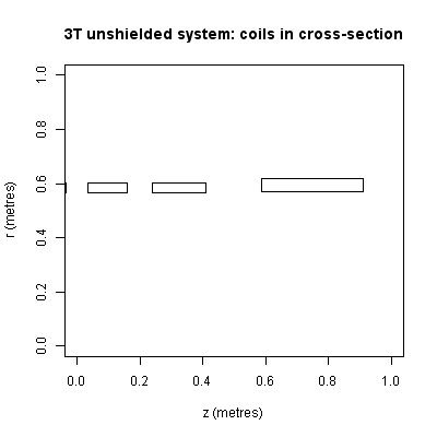 From the table of coil dimensions, the coils can be sketched in cross-section as shown. This is an unshielded magnet so the coils all have similar mean radius.
The coilset is symmetrical about the centreline.
The total length of the coils is around 2 x 0.9 metres or 1.8 metres.
If you ever need to have an MRI scan and wonder why you find yourself inside a long tubular space, it's because you are surrounded by the magnet coils. Don't worry, it's completely safe!
Zonal harmonics table for the 3T MRI magnet system
The table of zonal harmonics for the coils is shown next.
As the coilset is symmetrical about the centreline, the table shows just half of the coils, on the right hand side of the origin.
The field component harmonics are evaluated on a radius of 22.5cm, corresponding to the 45 cm DSV spec volume. The units are tesla per amp.
| coil | A[0,0] | A[2,0] | A[4,0] | A[6,0] | A[8,0] | A[10,0] |
|---|---|---|---|---|---|---|
| 4 | 2.007E-03 | -3.719E-04 | 4.905E-05 | -4.589E-06 | 1.365E-07 | 6.383E-08 |
| 5 | 1.942E-03 | 4.575E-05 | -4.898E-05 | 6.133E-06 | -1.153E-07 | -7.040E-08 |
| 6 | 1.931E-03 | 3.260E-04 | -7.160E-08 | -1.543E-06 | -2.102E-08 | 6.431E-09 |
| total | 5.880E-03 | -1.742E-07 | -1.410E-09 | 1.365E-09 | 2.459E-10 | -1.332E-10 |
| ppm | 1000000.00 | -29.63 | -0.24 | 0.23 | 0.04 | -0.02 |
| coil | A[12,0] | A[14,0] | A[16,0] | A[18,0] | A[20,0] |
|---|---|---|---|---|---|
| 4 | -2.009E-08 | 4.044E-09 | -6.678E-10 | 9.677E-11 | -1.268E-11 |
| 5 | 1.158E-08 | -7.704E-10 | -3.237E-11 | 1.483E-11 | -1.967E-12 |
| 6 | 1.265E-10 | -2.777E-11 | -6.055E-13 | 1.271E-13 | 2.848E-15 |
| total | -8.386E-09 | 3.246E-09 | -7.008E-10 | 1.117E-10 | -1.464E-11 |
| ppm | -1.43 | 0.55 | -0.12 | 0.02 | 0.00 |
The zonals table indicates that the operating current for a central field of 3 tesla is 255.12 amps. This may differ slightly from the operating current used in practice for technical reasons relating to the spectrometer radiofrequency settings.
The table also shows that the design is balanced to tenth order, as reported. The first effectively non-zero harmonic is twelfth. A significant amount of residual second order is present, but this would presumably be dealt with by the shimming process during system installation.
Field in the region of interest (ROI), 3T MRI magnet system
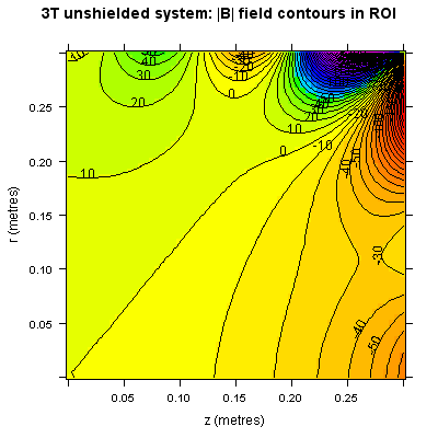 A contour plot of the field in the imaging region or region of interest (ROI) for the 3T MRI magnet system is shown. This is sometimes termed the magnetic field profile of the magnet.
Reddish tones indicate negative ridges whereas blue indicates positive ridges. The effects of the small residual 2nd order field component can be seen near to the origin but the general shape of the high-uniformity ROI is still evident.
Going from theta = zero to theta = 90 degrees on a constant radius, the magnetic field profile shows a series of alternating highs and lows. This is characteristic of MRI magnet systems (and magnets constructed from short solenoids in general).
Stray field contours
 Stray field contours are shown in the next plot. The 5 gauss contour extends further than in a typical active-shielded magnet (units for the plot are tesla: 5 G is equal to 5 10-4 T).
Inductance matrix for the 3T system
The inductance matrix for the magnet, calculated using Garrett's elliptic integral solver, is shown next. Units are henries. (Total inductance is 325.78 henries).
| [,1] | [,2] | [,3] | [,4] | [,5] | [,6] | |
|---|---|---|---|---|---|---|
| [1,] | 8.388E+01 | 9.434E+00 | 3.718E+00 | 2.385E+00 | 2.073E+00 | 2.788E+00 |
| [2,] | 9.434E+00 | 1.407E+01 | 4.380E+00 | 2.368E+00 | 1.820E+00 | 2.073E+00 |
| [3,] | 3.718E+00 | 4.380E+00 | 8.059E+00 | 3.562E+00 | 2.368E+00 | 2.385E+00 |
| [4,] | 2.385E+00 | 2.368E+00 | 3.562E+00 | 8.059E+00 | 4.380E+00 | 3.718E+00 |
| [5,] | 2.073E+00 | 1.820E+00 | 2.368E+00 | 4.380E+00 | 1.407E+01 | 9.434E+00 |
| [6,] | 2.788E+00 | 2.073E+00 | 2.385E+00 | 3.718E+00 | 9.434E+00 | 8.388E+01 |
Coil forces matrix for the 3T system
Next is the matrix of coil forces for the magnet. The units are newtons, so some of the forces are very large. The net force between either of the end coils (1 or 6) and the rest of the magnet is 3.26 meganewtons, or 332 tonnes force.
| [,1] | [,2] | [,3] | [,4] | [,5] | [,6] | |
|---|---|---|---|---|---|---|
| [1,] | 5.001E-10 | -1.782E+06 | -5.866E+05 | -3.377E+05 | -2.623E+05 | -2.913E+05 |
| [2,] | 1.782E+06 | -7.475E-12 | -1.058E+06 | -4.361E+05 | -2.862E+05 | -2.623E+05 |
| [3,] | 5.866E+05 | 1.058E+06 | 4.029E-11 | -9.185E+05 | -4.361E+05 | -3.377E+05 |
| [4,] | 3.377E+05 | 4.361E+05 | 9.185E+05 | 4.029E-11 | -1.058E+06 | -5.866E+05 |
| [5,] | 2.623E+05 | 2.862E+05 | 4.361E+05 | 1.058E+06 | -7.475E-12 | -1.782E+06 |
| [6,] | 2.913E+05 | 2.623E+05 | 3.377E+05 | 5.866E+05 | 1.782E+06 | 5.001E-10 |
| sum | 3.260E+06 | 2.600E+05 | 4.815E+04 | -4.815E+04 | -2.600E+05 | -3.260E+06 |